Example of Dynamic Analysis

Calculation Example. Dynamic analysis of cantilever beam with varying load

To illustrate functioning of dynamic analysis module let us consider an example of a cantilever rectangular beam with dimensions 1000х100х20. The material of the beam is steel AISI1020. The force is applied to the free end of the beam and is rising from 0 to 500 N for 2 sec, then it is constant and equal 500 N. Let us define the maximal displacements of the beam at the free loaded end and dynamic stresses in the fixed part of the beam. We will use both of dynamic analysis approach: Direct Time Integration and Mode Superposition and then compare the results.

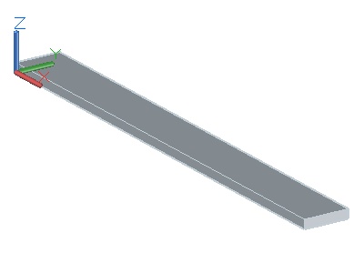
Example 3D model

Dynamic Transitional Process

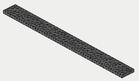
Step 1. Creation of study, creation of mesh, applying material. Use the command _FEMASTUDY to create the study on the basis of the body - beam with dimensions 1000х100х20. Create finite-element mesh. You need to define material parameters of the model. The physical properties exist in the AutoFEM base.

Created finite-element mesh

Step 2. Apply initial and boundary conditions. Initial conditions and loads should be specified. Initial conditions will be zero velocities and accelerations that need not be set separately. Apply full restraint to one end and vertical force that varies according to the graph to the other end.

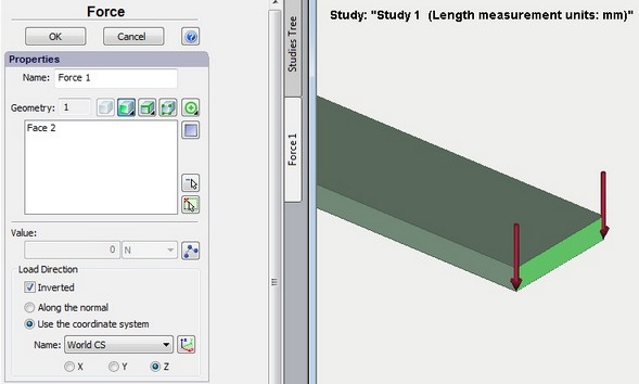
Varying load to the face

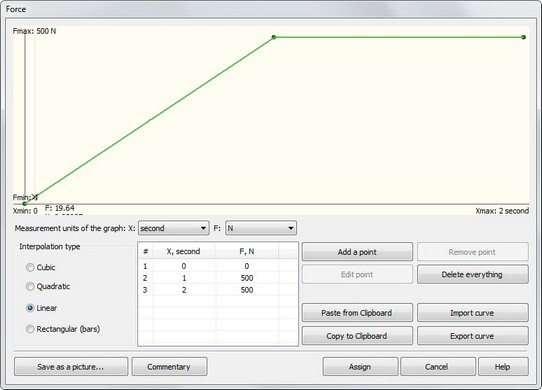
Graph of the varying load

Step 3. Creation of sensors and graphs templates. To define the maximum deflection and velocity of the beam end it is necessary to create sensor using which the graphs will be created:

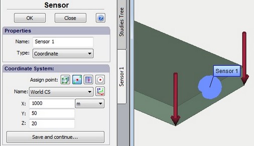
Sensor in the middle of the edge

Step 4. Solve Study. The study calculation is started after the restraints and loads are defined.

You should specify time step and finite time of the calculation in the study properties. According to the slow load change the 0.025 sec time step is defined.

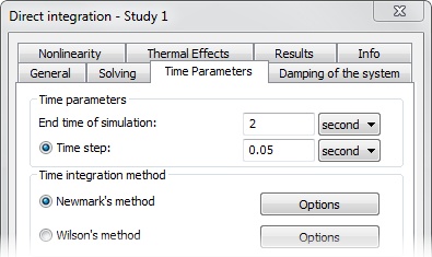
Specify step and time of the modelling

Step 5. Solving results analysis. After the calculation you need to open displacements result.

After "Time process" control pan activation we can watch the deformation process of the beam step by step. The beam will deform to the maximum value under the load and then the beam oscillates by inertia because it is still loaded with applied force. Oscillations are continuous so that the damping is not used in the study.

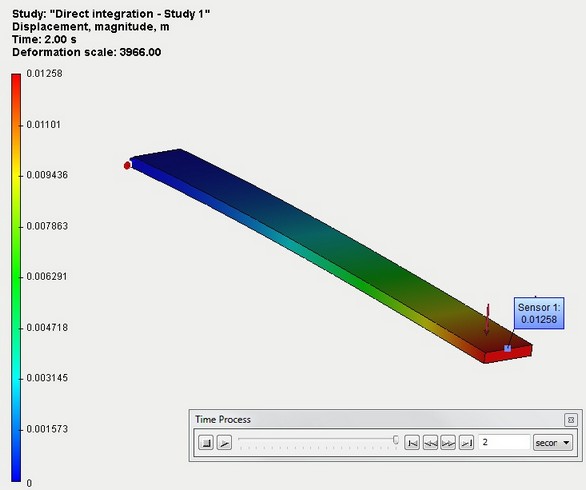
Displacements - time process

Deflection of the same beam under the constant force, received after static strength study calculation. The results practically coincide.

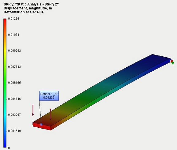
Comparison with the static displacement from the same static load

On the displacements graph created using Sensor_1 you may see that the beam end continues to oscillate with small amplitude with regard to the maximum deflection loaded with the applied force of 500 N.

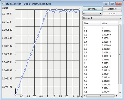
Displacements on the graph - time process

The maximal stresses can be shown on the stresses diagram. Display extremums. Make sure that received dynamic stresses are close to the stresses received in the static calculation.

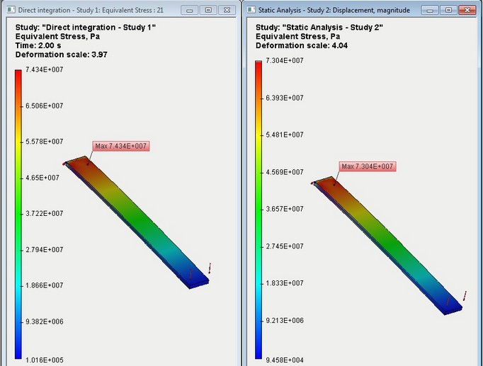
Comparison dynamic stresses (left) with static stresses

Mode Superposition

Calculate previous study using mode superposition (type: Mode Superposition).

Step 1. Creation or copying of the study. Use the_FEMASTUDY command to create the Frequency & Mode superposition study on the basis of the same beam or copy previous study and change its type to Mode superposition in the properties not to apply twice the same loads and restraints.

Step 2. Calculation of natural modes.

Select Calculate natural modes on the Solve tab in the study properties. The system offers to use 12 natural modes for the calculation.

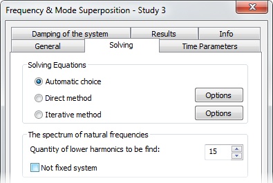
Specify the number of natural eigenmodes

Step 3. Solve Study. The study calculation is started after the restraints and loads are defined.

You should specify the same time step and finite time of the calculation as for the previous example in the study properties on the Parameters tab.

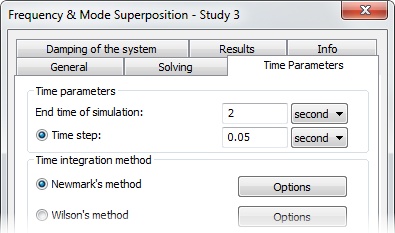
Specify step and time of the modelling

Step 4. Solving results analysis. After the calculation you need to open displacements result.

After the calculation is complete you should activate "Time process" control pan to watch the deformation process of the beam step by step. You can see that as for the Transitional process study the beam will deform under the load to the maximum value and then the beam oscillates by inertia with small amplitude near the maximum value of the deflection. The amplitude of the deflection practically coincide with the value found in the Transitional processes and Static strength studies.

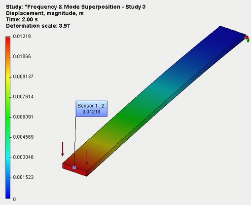
Dynamic displacements - time process

On the displacements graph created using Sensor_3 you may see that the beam end continues to oscillate with small amplitude with regard to the maximum deflection.

Oscillations are continuous so that the damping is not used in the study.

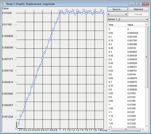
Displacements - time process

When extrema are displayed on the stresses diagram you can see that the computation stresses are close by their values to the previously calculated values.

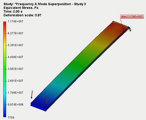
Dynamic stresses in the Mode superposition

Conclusion:

According to the solved study you may see that both of the methods of dynamic study calculation lead to the same result and can be used for the dynamic analysis of structures.

Return to contents

autofem.com