| AutoFEM Analysis Settings of Linear and Nonlinear Statics Processor | |||||||
| AutoFEM Analysis Settings of Linear and Nonlinear Statics Processor | |||||||
Settings of Linear and Nonlinear Statics Processor
The user-defined study properties are saved together with the document and are inherited upon copying a study. The main purpose of the study properties is defining options required for the processor, the result listings to be displayed after completing calculations in the studies tree, as well as keeping the descriptive attributes of the study, as the name or a comment. The static analysis solution parameters dialogue has five tabs.
The [General] tab serves for defining descriptive properties of the current study.
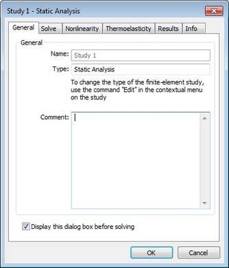
In the "Name" field, the user can edit the study name assigned the system default at creation. This name will be further on displayed in the studies tree, in the results window and in the report. The "Type" control serves for defining the study type. Note that AutoFEM allows changing an existing study type to another one from the list of study types available to the user. For example, the user can create a study of the "Static Analysis" type, and then change the type, for example, to "Stability" or "Frequency analysis".
The "Comment" edit box lets the user entering arbitrary text information pertaining to the current study. This information will be used in the future for generating a report based on the study solution results.
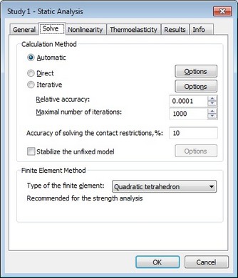
The [Solve] tab serves for defining processor properties for solving linear statics equations. The control elements in the "Calculation method" group lets the user define the methods of solving systems of algebraic equations of linear statics.
Automatic. The solver chooses the method of solving equations based on the number of equations. If the number of equations exceeds the threshold set in the Account Settings AutoFEM (the default is set to 100.000), the system of equations is solved by an iterative method, if the number of equations is less than the specified limit, the direct method of solution is chosen .
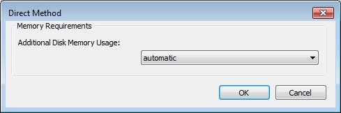
Direct method. The system of equations is solved by Gauss method via LU decomposition of the stiffness matrix. This method is effective for solving the system of equations constructed on the basis of the linear finite elements. In certain cases, the use of direct method can be also justified for analysis of the system with the help of quadratic finite elements. It can be used instead of iterative method, if the iterative algorithm does not converge to the stable solution, or if the convergence speed is very small (the number of iterations is several thousands). This situation can be observed for «thin» problems (the model is flat or stretched), and also, for a large number of finite elements which are considerably different from equilateral elements (when the ratio of the lengths of the finite element edges are on the order of hundreds or thousands). Additional settings of the direct method are available (button "Options")
Iterative. The systems of equations are solved by iterative methods. This method is used by default for solving systems of equations, built based on a quadratic finite element. The following two options can be set for the iterative method: relative tolerance and the maximum number of iterations. Additional settings of the iterative method are available ("Options")
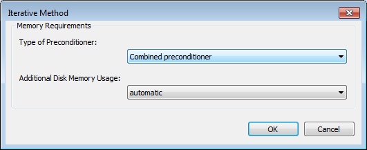
Additional disk memory usage. The user can also manage interaction with external (disk) memory of the computer system when solving equations by a direct or iterative method ([Options]). There are three options for using additional disk memory: automatic, not available, mandatory. The use of additional disk memory allows you to save the stiffness matrix decomposition.Using additional disk memory for solving systems of equations is necessary only when the memory requirement for keeping intermediate matrixes exceeds the computer's RAM. Note also that the running time for studies with a large number of dimensions using external storage could be significant due to a large number of operations on sequential data read-write.
High volumes of disk storage may be needed for keeping intermediate matrixes (up to several Gigabytes). Make sure there is enough disk space before solving studies in large dimensions using external storage.
If the user disabled the possibility of using the disk space while solving a high order system of equations, an abnormal termination of the process may abort calculations in the event of the memory consumption for keeping the matrix decomposition approaching 2 Gigabyte (for Windows 32-bit).
Type of Preconditioner (for iterative method). Four types of preconditioners are available. Combined Preconditioner is the fastest and default method. It consumes maximal amount of memory. Incomplete Decomposition, it takes an additional memory, which amount is equal the memory, occupied by the stiffness matrix. Diagonal and Identity Preconditioner, they practically not use additional memory, but provide a lowest rate of convergence.
Relative accuracy - the accuracy of the achieved iterative solution. The smaller is the specified miscalculation error, the greater number of steps (iterations) will be required.
Maximum number of iterations - the critical number of iterations, after reaching which the iterative solving of the system of equations terminates, even if the required solution precision was not achieved.
Accuracy of solving contact restrictions. This parameter specifies the relative percentage of the contacting nodes that are excluded at each step of the iterative process during the calculation of contact boundary conditions. The minimum value is 1%, maximum 50%. From the point of view of the user, a smaller value slows down the solution of the contact problem, although the accuracy of the solution is increased.
Stabilize the unfixed model. Usually, the static strength calculation of unfixed model, which is balanced only by the forces, is impossible. Due to rounding errors the model is shifted in space or rotates. These displacements are significantly larger than deformations occurring in the model as a result of static forces action and do not allow us to estimate the stress-strain state of the system. This flag turns on the stabilization of the unfixed model in space. The principle of the stabilization is as follows. On all facets of the model are applied imaginary soft springs. It is assumed that the stiffness of the springs is negligible compared with the stiffness of the material from which the body was made. Therefore, they do not affect significantly on the result of static calculation. But this springs do not allow the model to move uncontrollably in space. The user can choose an acceptable value of stiffness to stabilize the system in each practical case.
Finite-Element Method. By default, all calculations use quadratic approximation for displacements, regardless of what kind of finite element mesh was constructed for the model. If the user is only interested in qualitative results, that is, he is only interested in relative distribution of stress fields, using a rather fine mesh, then one can use the linear element solution, which runs much faster than the quadratic counterpart. The hybrid element is used for static strength analysis of the models containing both linear plate-like and 3D volume elements (so called «hybrid» models).
Note! The linear tetrahedral finite element provides insufficient accuracy of quantitative results. Maximum displacement and stress results are much smaller via the calculation by linear tetrahedral finite elements, rather than those achieved by more accurate methods. It is strongly recommended to use quadratic element calculations for quantitative evaluation (the default mode).
The [Thermoelasticity] tab allows to define the methods for calculating thermal loads.
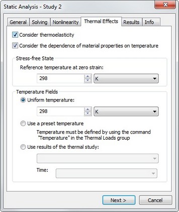
Consider Thermoeffects. Includes the mode of calculating loads building up in a structure due to the linear expansion forces under the condition of heat applied to the body.
Temperature of zero deformations: - the initial body temperature, at which there is no thermal strain and there is no stress caused by difference in temperatures. The user can specify temperature values in one of the existing scales: K - Kelvins; C - Celsius; F- Farenheit. Define the method of specifying thermal loads in the "Temperature fields" group.
Uniform temperature - the value of a uniform temperature field is specified in the chosen units, which affects all studied bodies.
Use preset temperature - thermal loads are included in the static analysis, that were defined by the command "AutoFEM | Loads / Restraints | Temperature".
Use heat-task results - available solution of the thermal analysis study is used for defining the thermal loading. In the drop-down list select the name of the solved thermal analysis study and (if necessary) the time instant, to which the solution pertains. Please note that certain conditions are to be met for using thermal analysis results as the initial temperature conditions:
1.Identity condition of finite element meshes in static and thermal analyses. The simplest way of achieving such identity is the use of the "Copy" command available in the context menu. The sequence of steps can be, for example, as follows:
a) Create a study of the type "Thermal Analysis", generate a mesh, define boundary conditions, and run;
b) Create a study copy using the "Copy" command;
c) On the tab "General" in the study properties dialogue, changed the study type to "Static Analysis".
As a result, we have two studies of different types, but with identical finite element meshes.
2.The "Calculate using linear element" property on the "Solve" tab of the study parameters dialogue should use the same settings in both studies. For example, if the thermal analysis is done by linear elements, then the static analysis based on thermal analysis results can also be run only by linear elements.
The [Results] tab allows defining the result types displayable in the studies tree after finishing calculations.
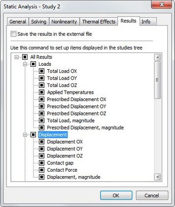
Save solving results in file - enables the mode, in which all analysis results are saved in the file together with the model. This allows analysing results of an earlier calculated and saved study without the need for a new calculation. Please note that saving calculation results in a document increases the size of the document file by approximately 4.5 to 5 Mbyte per a hundred thousand Degrees of Freedom.
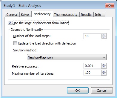
The tab [Nonlinear] allows the user to carry out statical analysis taking into consideration large displacements.
In practice, there are situations in which displacements of certain points of the structure reach significant values under the action of external loads. These problems are especially important in aircraft and space industry, when designing radio-telescopes, cooling towers and other thin-walled structures. In these cases the nonlinear effects should be taken into consideration, since the assumptions on which the linear analysis is built are not valid.
The option "Use large displacement formulation" should be activated in cases when at least one of the following assumptions of the linear analysis is violated:
1. Resulting deformations are sufficiently small, so the stiffness changes caused by the load can be ignored;
2. In the process of applying the load, boundary conditions do not change amplitude, direction and distribution.
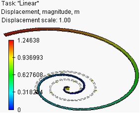
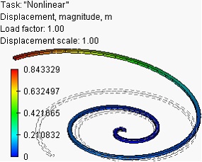
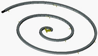
For example, the linear analysis of the spiral-like part subject to the load applied at the end edge gives an error of approximately 30% compared to the nonlinear analysis. This difference in results arises due to small displacement assumption adopted in linear analysis.
|
|
Linear analysis |
Nonlinear analysis |
Controls in the group «Geometric nonlinearity» allow the user to customize the process of solution of geometrically nonlinear problems.
For solving such problems, a time stepping nonlinear solver organizes the process of incremental loading of structure and gives the solution of the linearized system of equations at each step for the current increment of the load vector, formed for a specific loading.
Number of load steps. This option allows the user to set the number of steps during which the load will be changing from zero to a specified value. Theoretically, all solutions can be found within one step for total value of acting load. However, there arises the possibility of non-uniqueness of solution, and, moreover, the found solution may not have physical meaning. In such cases, it is reasonable to specify the load incrementally and obtain nonlinear solution for each increment. From the computational point of view, it is often efficient because the nonlinear effects will be getting smaller at each step. If the increments of load are sufficiently small in magnitude, each incremental solution can be found within one step with a high degree of accuracy. By default, the number of steps is set to 10.
Update load direction allows the user to account for change in the load vector, while applying the loading, according to the deformed geometry of the model.
Solution method. By default, the Newton-Raphson method of solving the system of nonlinear equations is used. At each step of load application, the system of the linear algebraic equations is being solved until the relative error between two consecutive solutions does not become smaller than the prescribed tolerance.
If the number of iterations reaches the value larger than the specified one, the calculations are terminated.
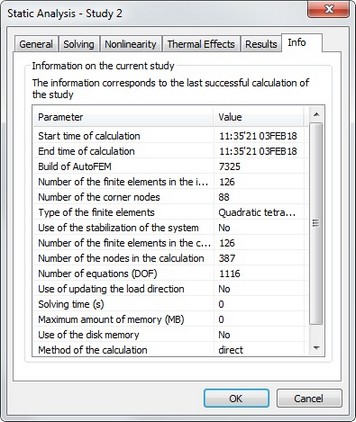
The tab [Info] contains main information about the solved study - date of solving, memory consumption, number of finite elements and equations and other useful data.