| AutoFEM Analysis Settings of Buckling Analysis Processor | |||||||
| AutoFEM Analysis Settings of Buckling Analysis Processor | |||||||
Buckling Analysis Processor Settings
Upon initializing the "AutoFEM | Solve..." command, the dialogue of defining study properties appears by default, with several tabs to switch between. The user can change the default study properties. To access a study's properties, click ![]() on the name of the selected study in the AutoFEM Palette window. The user-defined study properties are saved together with the document and are inherited upon copying a study. The main purpose of this study properties is defining the modes of the Processor's operation, as well as the lists of results and the number of buckling modes displayable in the studies three after calculations.
on the name of the selected study in the AutoFEM Palette window. The user-defined study properties are saved together with the document and are inherited upon copying a study. The main purpose of this study properties is defining the modes of the Processor's operation, as well as the lists of results and the number of buckling modes displayable in the studies three after calculations.
On the [General] tab, you can see or modify the descriptive properties of the current study: the name, the study type, the comment.
On the [Solve] tab, you can define processor properties for solving the equations.
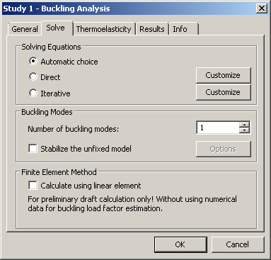
In the group « Solving Equations » the method of solving equations can be set.
Automatic choice - the method of solving equations is selected automatically according to overall number of equations. The threshold is set in Settings | Processor. The default value is set equal 100,000. If the total number of equations exceed defined value, the iterative method of solving equations is used. Otherwise, direct method will be used.
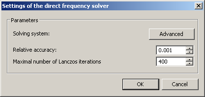
Direct - this method uses full inversion of the matrix to find the factor of critical load, therefore, it usually requires more random memory than iterative method. It works fairly fast for solving relatively small problems and on powerful computer systems. The button "Customize" in front of the option opens the dialogue box of calculation settings:
Relative accuracy of solution, after reaching which the iterative process terminates.
Maximal number of Lanczos iterations - the critical number of iterations, after reaching which the iterative solving of the system of equations terminates, even if the required solution precision was not achieved.
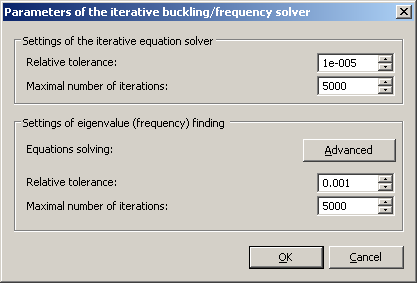
Iterative - this method has lower memory requirements than direct method because the inversion of matrix is not carried out. It allows to solve large buckling problems. The rate of convergence (solving time) linearly depends on the quantity of desired buckling modes. Also, the rate of solving is sensitive to quality of finite element mesh. When the mesh has significant quantity stretched finite element (tetrahedrons or triangles) the rate of convergence may decrease (solving time increase). The button "Customize" opens the dialogue box of calculation settings. The group "Settings of the iterative equation solver" contains parameters Relative tolerance and Maximal number of iterations of the linear equation solver used for solving the static analysis study which precedes the buckling study solving. The group "Settings of eigenvalue (frequency) finding" contains the parameters of the iterative eigenvalue solver, such as Relative tolerance and Maximal number of iterations.
In the group «Parameters of Analysis» the user can set following options:
Number of buckling modes. The user can specify the number of critical loads and respective buckling modes to be identified. For practical purposes, the most important is the first mode, corresponding to the minimum critical load. Nevertheless, the user may also find the critical loads of other buckling modes.
In the group «Finding State Forms» for parameter «Solving System», it is required to indicate possibility of using additional disk memory ([Customize]): automatic, not available, mandatory. The use of additional disk memory allows the user to save decomposition of the stiffness matrix on the disk.
Relative tolerance – the accuracy of determining critical loads; upon reaching this accuracy, the iterative process stops.
Maximum number of iterations - the critical number of iterations, after reaching which the iterative solving of the system of equations terminates, even if the required solution accuracy was not achieved.
Stabilize the unfixed model. Usually, the buckling analysis of unfixed model, which is balanced only by the forces, is impossible. Due to rounding errors the model is shifted in space or rotates. These displacements are significantly larger than deformations occurring in the model as a result of static forces action and do not allow us to estimate the stress-strain state of the system. This flag turns on the stabilization of the unfixed model in space. The principle of the stabilization is as follows. On all facets of the model are applied imaginary soft springs. It is assumed that the stiffness of the springs is negligible compared with the stiffness of the material from which the body was made. Therefore, they do not affect significantly on the result of stress calculation. But this springs do not allow the model to move uncontrollably in space. The user can choose an acceptable value of stiffness to stabilize the system in each practical case.
In the group “Finite-Element Method" the user can set the mode «Calculate using linear element». This facilitates much faster calculation for an approximate estimate of the buckling mode amplitudes relative distribution on a sufficiently fine mesh.
The linear tetrahedral finite element provides insufficient accuracy of calculating critical loads. Critical load results are much greater (by a factor of tens or hundreds of times) via the calculation by linear finite elements, rather than those achieved by more accurate methods. It is strongly recommended to use only quadratic element calculations for quantitative evaluation of the critical loads (the default mode). |
The [Thermoelasticity] tab allows to define the methods for calculating thermal loads. Its settings are completely coincide with settings of Thermoelasticity in static analysis
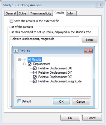
The [Results] tab sets the displayable result types in the studies tree after finishing calculations.